and the distribution of digital products.
The Theory of Econometric Duality
:::info Author:
(1) David Staines.
:::
Table of Links4 Calvo Framework and 4.1 Household’s Problem
4.3 Household Equilibrium Conditions
4.5 Nominal Equilibrium Conditions
4.6 Real Equilibrium Conditions and 4.7 Shocks
5.2 Persistence and Policy Puzzles
6 Stochastic Equilibrium and 6.1 Ergodic Theory and Random Dynamical Systems
7 General Linearized Phillips Curve
8 Existence Results and 8.1 Main Results
9.2 Algebraic Aspects (I) Singularities and Covers
9.3 Algebraic Aspects (II) Homology
9.4 Algebraic Aspects (III) Schemes
9.5 Wider Economic Interpretations
10 Econometric and Theoretical Implications and 10.1 Identification and Trade-offs
10.4 Microeconomic Interpretation
\ Appendices
A Proof of Theorem 2 and A.1 Proof of Part (i)
B Proofs from Section 4 and B.1 Individual Product Demand (4.2)
B.2 Flexible Price Equilibrium and ZINSS (4.4)
B.4 Cost Minimization (4.6) and (10.4)
C Proofs from Section 5, and C.1 Puzzles, Policy and Persistence
D Stochastic Equilibrium and D.1 Non-Stochastic Equilibrium
D.2 Profits and Long-Run Growth
E Slopes and Eigenvalues and E.1 Slope Coefficients
E.4 Rouche’s Theorem Conditions
F Abstract Algebra and F.1 Homology Groups
F.4 Marginal Costs and Inflation
G Further Keynesian Models and G.1 Taylor Pricing
G.3 Unconventional Policy Settings
H Empirical Robustness and H.1 Parameter Selection
I Additional Evidence and I.1 Other Structural Parameters
I.3 Trend Inflation Volatility
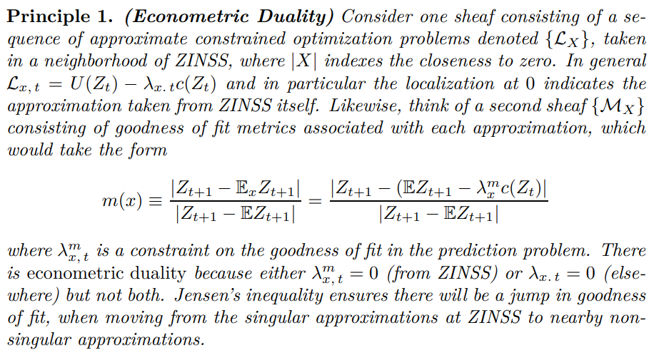
10.2 Econometric DualityThis crucial subsection uncovers the deep connection between the topology and goodness of fit of approximate solutions around ZINSS. I finish by discussing bias implications to stimulate future computational and econometric work. The key idea is that missing dynamics in the existing approximation can directly translate to poor econometric performance.
10.2.1 Theoretical FormulationThis part sets out the mathematical foundation for the econometric analysis.
\

\

\ Remark 34. Different bifurcation experiments correspond to different sheaves. It is convenient to work with the following parametization X = (δ, n, m) where δ is the starting rate of trend inflation, n is the order of the initial difference between stochastic and non-stochastic steady states and m is the limiting order of perturbation. Thus the |ε| limit would (0, 2, 1), √ ε would be (0, 2, 1/2). The first order non-stochastic bifurcation would be (δ, 0, 1), with (δ, 0, n) the corresponding bifurcation at a general order of approximation n.
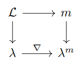
\ There are two informative visual representations. The first is the commuting diagram below where ∇ is the duality map and dependence on X has been suppressed.
\

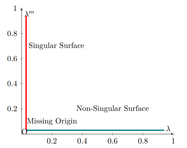
\ ∇ is anti-symmetric and it can be represented by the following correspondence. It represents a morphism between the sheaf of local goodness of fit metrics around ZINSS and the sheaf of approximate optimization problems, through their constraints.[93] The correspondence can be represented graphically as shown above. The hole at the origin is a consequence of Divine Coincidence. There is an unacceptable trade-off between simplifying the model by cancelling lag terms and fitting the data.
10.2.2 DiscussionDuality justifies the terminology of the boundary surface. It represents constraints that are always binding on the representative firm / social planner or the econometrician. This principle demonstrates a direct connection between the microfoundations missing from the faulty approximations at ZINSS and its poor empirical performance. If we believe in our Keynesian microfoundations we should expect a substantial improvement in goodness of fit when we change to the correct approximation. This is a reassuring prospect. The general conclusion is surely that modern Keynesian economics is first and foremost about justifying the presence of lags in the Phillips Curve, operating through the constraints implied by staggered optimization. Previous approximations failed to represent the underlying microfoundations; as such they failed the Lucas critique.
\

\ Econometric duality is a theoretical result that holds under the null hypothesis the model is true. If the real data generating process is sufficiently close to the theory the associated improvement in goodness of fit will still arise. This is an econometric hypothesis. However, on the basis of the exercise in Section 3.1 and Appendix H, I will proceed as though it is true that (2) fits the data better than (1).
\ This can seriously bias inference, drawn from goodness of fit comparisons. Suppose an econometrician were trying to estimate the improvement in the goodness of fit associated with a change like modelling (non-zero) trend inflation Zπ but were unaware of the bifurcation. They would use the estimator
\

\ for the appropriate (convergent) goodness of fit metric k·| k but the true improvement would be
\

\ This yields an upward bias in the inferred improvement in the goodness of fit.
\

\ It would distort hypothesis testing towards accepting ill-fitting alternatives to the benchmark Calvo model. This would extend to any alternative to the Calvo that did not suffer from the same singularity. This would include alternative pricing models, such as those with Taylor [1979] or menu costs.
\ In fact any bifurcation will cause overestimation of non-linearity nearby a faulty linearized benchmark. The theory is as follows: an econometrician wishing to estimate the non-linearity compared to the singular solution would estimate
\

\ the true estimator would be
\

\ thus an asymptotic bias would emerge
\

\ It is strictly positive if the true non-linearity is small. It remains to test whether this approximate bound holds in simulations. Nevertheless, the a priori case was typically avoided, now at the expense of irrelevance, by using Rotemberg pricing.[94] In theory for ex post bifurcation the bias would be infinite in any neighborhood of the cut-off as calculated for Calvo in the next section. An underlying theme is that complicated singularities are not amenable to inferential statistical learning. The confusion should now be over.
\
:::info This paper is available on arxiv under CC 4.0 license.
:::
[93] Or even a functor between the two categories of sheaves around ZINSS, as in Appendix F.2.
- Home
- About Us
- Write For Us / Submit Content
- Advertising And Affiliates
- Feeds And Syndication
- Contact Us
- Login
- Privacy
All Rights Reserved. Copyright , Central Coast Communications, Inc.