Stable Diffusion is a LDM, operating in a pretrained, learned (and fixed) latent space of an autoencoder. While the bulk of the semantic composition is done by the LDM [38], we can improve local, high-frequency details in generated images by improving the autoencoder. To this end, we train the same autoencoder architecture used for the original Stable Diffusion at a larger batch-size (256 vs 9) and additionally track the weights with an exponential moving average. The resulting autoencoder outperforms the original model in all evaluated reconstruction metrics, see Tab. 3. We use this autoencoder for all of our experiments.

\ Stable Diffusion 2.x uses an improved version of Stable Diffusion 1.x’s autoencoder, where the decoder was finetuned with a reduced weight on the perceptual loss [55], and used more compute. Note that our new autoencoder is trained from scratch.

2.5 Putting Everything Together

We train the final model, SDXL, in a multi-stage procedure. SDXL uses the autoencoder from Sec. 2.4 and a discrete-time diffusion schedule [14, 45] with 1000 steps. First, we pretrain a base model (see Tab. 1) on an internal dataset whose height- and width-distribution is visualized in Fig. 2 for 600 000 optimization steps at a resolution of 256 × 256 pixels and a batch-size of 2048, using sizeand crop-conditioning as described in Sec. 2.2. We continue training on 512 × 512 pixel images for another 200 000 optimization steps, and finally utilize multi-aspect training (Sec. 2.3) in combination with an offset-noise [11, 25] level of 0.05 to train the model on different aspect ratios (Sec. 2.3, App. I) of ∼ 1024 × 1024 pixel area.

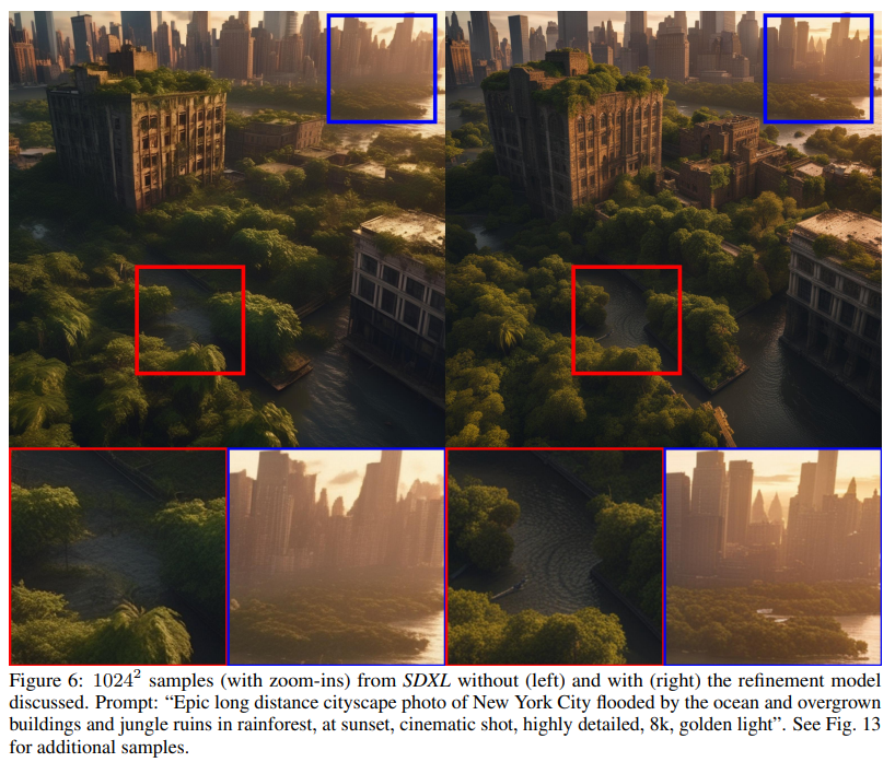
\ Refinement Stage Empirically, we find that the resulting model sometimes yields samples of low local quality, see Fig. 6. To improve sample quality, we train a separate LDM in the same latent space, which is specialized on high-quality, high resolution data and employ a noising-denoising process as introduced by SDEdit [28] on the samples from the base model. We follow [1] and specialize this refinement model on the first 200 (discrete) noise scales. During inference, we render latents from the base SDXL, and directly diffuse and denoise them in latent space with the refinement model (see Fig. 1), using the same text input. We note that this step is optional, but improves sample quality for detailed backgrounds and human faces, as demonstrated in Fig. 6 and Fig. 13.

\ To assess the performance of our model (with and without refinement stage), we conduct a user study, and let users pick their favorite generation from the following four models: SDXL, SDXL (with refiner), Stable Diffusion 1.5 and Stable Diffusion 2.1. The results demonstrate the SDXL with the refinement stage is the highest rated choice, and outperforms Stable Diffusion 1.5 & 2.1 by a significant margin (win rates: SDXL w/ refinement: 48.44%, SDXL base: 36.93%, Stable Diffusion 1.5: 7.91%, Stable Diffusion 2.1: 6.71%). See Fig. 1, which also provides an overview of the full pipeline. However, when using classical performance metrics such as FID and CLIP scores the improvements of SDXL over previous methods are not reflected as shown in Fig. 12 and discussed in App. F. This aligns with and further backs the findings of Kirstain et al. [23].

:::info This paper is available on arxiv under CC BY 4.0 DEED license.

:::

Feed: Hacker Noon - Medium

View: Original article

Tags: distribution

Content Distribution