and the distribution of digital products.
How Firms Set Prices and Adjust for Inflation: The Basics of Calvo Pricing
4 Calvo Framework and 4.1 Household’s Problem
4.3 Household Equilibrium Conditions
4.5 Nominal Equilibrium Conditions
4.6 Real Equilibrium Conditions and 4.7 Shocks
5.2 Persistence and Policy Puzzles
6 Stochastic Equilibrium and 6.1 Ergodic Theory and Random Dynamical Systems
7 General Linearized Phillips Curve
8 Existence Results and 8.1 Main Results
9.2 Algebraic Aspects (I) Singularities and Covers
9.3 Algebraic Aspects (II) Homology
9.4 Algebraic Aspects (III) Schemes
9.5 Wider Economic Interpretations
10 Econometric and Theoretical Implications and 10.1 Identification and Trade-offs
10.4 Microeconomic Interpretation
\ Appendices
A Proof of Theorem 2 and A.1 Proof of Part (i)
B Proofs from Section 4 and B.1 Individual Product Demand (4.2)
B.2 Flexible Price Equilibrium and ZINSS (4.4)
B.4 Cost Minimization (4.6) and (10.4)
C Proofs from Section 5, and C.1 Puzzles, Policy and Persistence
D Stochastic Equilibrium and D.1 Non-Stochastic Equilibrium
D.2 Profits and Long-Run Growth
E Slopes and Eigenvalues and E.1 Slope Coefficients
E.4 Rouche’s Theorem Conditions
F Abstract Algebra and F.1 Homology Groups
F.4 Marginal Costs and Inflation
G Further Keynesian Models and G.1 Taylor Pricing
G.3 Unconventional Policy Settings
H Empirical Robustness and H.1 Parameter Selection
I Additional Evidence and I.1 Other Structural Parameters
I.3 Trend Inflation Volatility
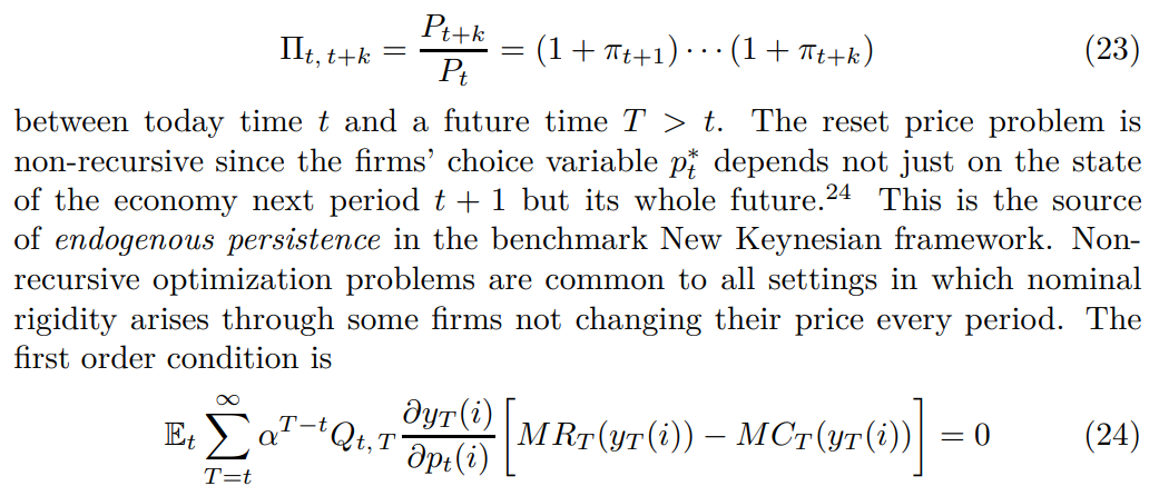
4.4 Price-Setting ProblemCalvo [1983] pricing is the most popular approach to inject nominal rigidity into a DSGE model. Re-optimization is governed by a stochastic process common across firms. With probability 1 − α each firm is free to reset its price (at no cost), whilst with probability α it keeps its price fixed and meets demand at its existing price. Firms reset their prices to maximize the expected present value of profits through the lifetime of the price as follows:
\

\ subject to the individual demand (17). Here
\

\ represents the real stochastic discount factor (SDF). It is the risk-adjusted present value of future consumption k periods ahead which depends on the gross rate of inflation
\

\ It states that optimal pricing sets a weighted stream of marginal revenues equal to a weighted stream of marginal costs, which in turn implies a similar relationship between (real) price and marginal costs
\

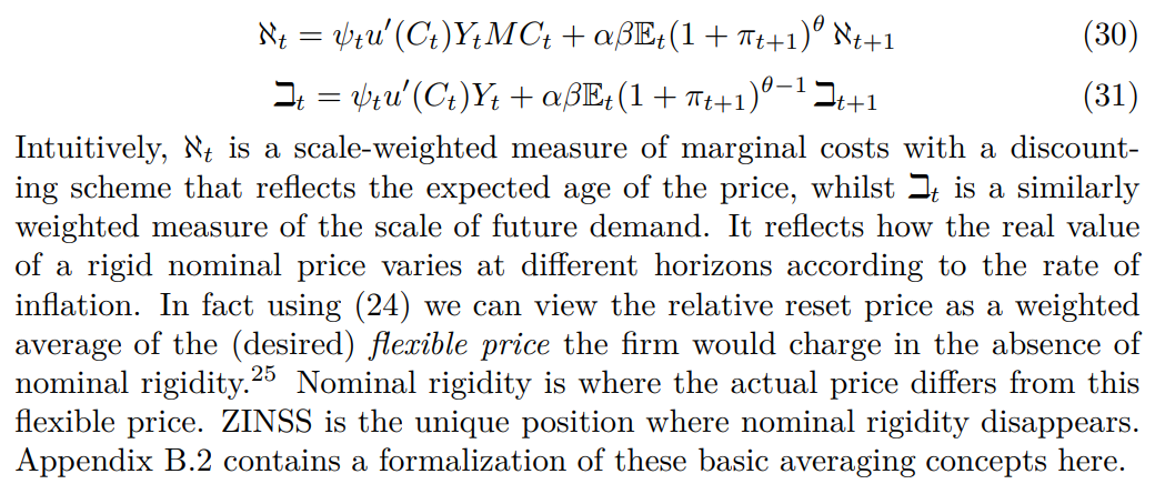
\ The persistence of the price level depends on α the degree of price rigidity. The reset price can be expressed as
\

\ where
\

\ both numerator and denominator have recursive forms
\

\ The first elementary result settles the connection between the relative reset price and the rate of inflation, central to the interpretation of the bifurcation.
\

\ Proof. Using (26) establishes that
\
\

\ The result follows from taking and signing the derivative
\

:::info Author:
(1) David Staines.
:::
:::info This paper is available on arxiv under CC 4.0 license.
:::

- Home
- About Us
- Write For Us / Submit Content
- Advertising And Affiliates
- Feeds And Syndication
- Contact Us
- Login
- Privacy
All Rights Reserved. Copyright , Central Coast Communications, Inc.