and the distribution of digital products.
How to Find the “Routes” of All-Pairs Shortest Paths With the Floyd-Warshall Algorithm in C#
In the previous post, we saw how to solve the all-pairs shortest path problem using the Floyd-Warshall algorithm. We also explored several ways to improve the algorithm’s performance by using parallelism and vectorization.
\ However, if you think about the results of the Floyd-Warshall algorithm, you will quickly realise the interesting moment – we know the distances (values of shortest paths) between vertexes in a graph but we don’t know the “routes” i.e., we don’t know what vertexes contribute to each shortest path, and we can’t rebuild these “routes” from the results we have.
\ In this post, I invite you to join me and extend the Floyd-Warshall algorithm. This time, we are going to make sure we can calculate the distance and rebuild the “route.”
A Bit of Known Theory…Before diving into code and benchmarks, let’s revise a theory of how the Floyd-Warshall algorithm works.
\ Here is a textual description of the algorithm:
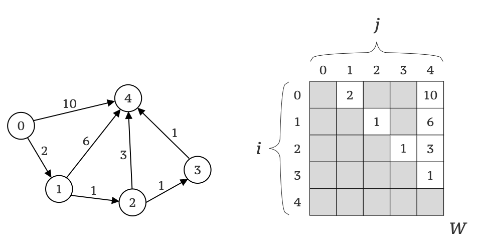
We start by representing a graph (G) of size N as matrix (W) of size N x N where every cell W[i,j] contains the weight of an edge from vertex i to vertex j (see Picture 1). In cases when there is no edge between vertexes, the cell is set to a special NO_EDGE value (shown as dark cells in Picture 1).
\
From now on, we say – W[i,j] contains a distance between vertexes i and j.
\
Next, we take a vertex k and iterate through all pairs of vertexes W[i,j] checking if distance i ⭢ k ⭢ j is smaller than the currently known distance between i and j.
\
The smallest value is stored in W[i,j] and step #3 is repeated for the next k until all vertexes of G have been used as k.
\
\ Here is the pseudo-code:
algorithm FloydWarshall(W) do for k = 0 to N - 1 do for i = 0 to N - 1 do for j = 0 to N - 1 do W[i,j] = min(W[i,j], W[i,k] + W[k,j]) end for end for end for end algorithmWhen done, every cell W[i,j] of matrix W either contains a distance of the shortest path between vertexes i and j or a NO_EDGE value, if there is no path between them.
\ As I mentioned in the beginning – having only this information makes it impossible to reconstruct the routes between these vertexes. So… what should we do to be able to reconstruct these routes?
\ Well… it may sound obvious but… we need to collect more data!
… A Bit of the Same Theory but From a Different AngleThe essence of the Floyd-Warshall algorithm is a compartment of known distance W[i,j] with a distance of potentially new path from i to j through intermediate vertex k.
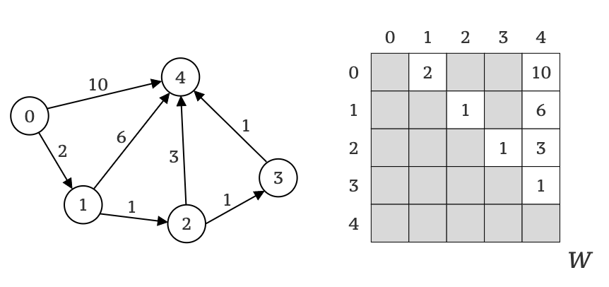
\ I drag so much attention to this detail because it is the key to how we can preserve route information. Let’s take the previous graph of 5 vertexes (see Picture 2) and execute the Floyd-Warshall algorithm on it.
\
\ Initially, we know about all graph edges, which gives us the following paths: 0 ⭢ 1 :2, 0 ⭢ 4 :10, 1 ⭢ 3 :1, 2 ⭢ 4 :1, 3 ⭢ 2 :1 and 3 ⭢ 4 :3.
:::tip I use the “from” ⭢ “to” :”distance” format from the previous post to write down paths.
\ - Author’s note
:::
We also know there are no edges leading to vertex 0, so executing an algorithm for k = 0 makes no sense. It is also obvious, there is a single edge (0 ⭢ 1) leading to from vertex 0 to vertex 1, which also makes the execution of all i != 0 (the i is “from” here) quite meaningless and because vertex 1 has edges with 2 and 4, it also makes no sense to execute algorithms for any j which isn’t 2 or 4 (the j is “to” here).
\ That is why our first step will be to execute an algorithm for k = 1, i = 0 and j = 2,4.
\
| Step | Path | Comment | |----|----|----| | 1 | 0 ⭢ 1 ⭢ 2 | Path found. Distance = 3 (was nothing) | | 2 | 0 ⭢ 1 ⭢ 4 | Path found. Distance = 8 (was 10). |
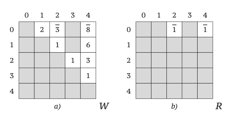
\ We have found two paths: a new path (0 ⭢ 1 ⭢ 2) and a shortcut (0 ⭢ 1 ⭢ 4). Both go through vertex 1. If we don’t store this information (the fact we got to 2 and 4 through 1) somewhere right now, it will be lost forever (and that is quite the opposite of what we want).
\ So what should we do? We will update matrix W with new values (see Picture 3a) and also store the value of k (which is k = 1) in cells R[0,2] and R[0,4] of a new matrix R of same size as matrix W but initialized with NO_EDGE values (see Picture 3b).
\
\ Right now, don’t focus on what exactly matrix R is. Let’s just keep going and execute the algorithm for the next k = 2.
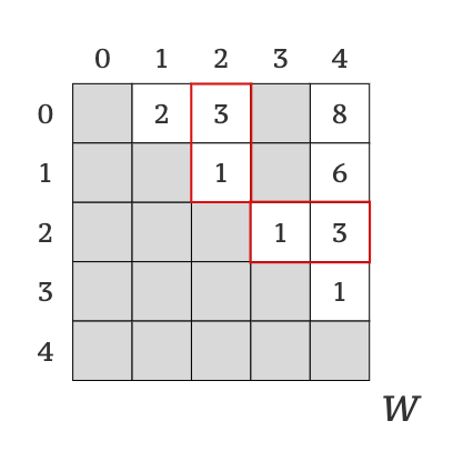
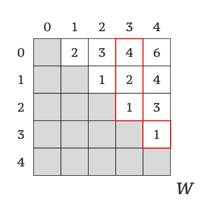
\ Here, we will do the same analysis (to understand what combinations make sense to execute) as we did for k = 1, but this time, we will use matrix W instead of graph G. Look at the matrix W, especially in column #2 and row #2 (Picture 4).
\
\ Here you can see, there are two paths to vertex 2 from vertex 0 and from vertex 1 (column #2), and two paths from vertex 2 to vertex 3 and to vertex 4 (row #2). Knowing that, it makes sense to execute the algorithm only for combinations of k = 2, i = 0,1 and j = 3,4.
\
| Step | Path | Comment | |----|----|----| | 1 | 0 ⭢ 2 ⭢ 3 | Path found. Distance = 4 (was nothing) | | 2 | 0 ⭢ 2 ⭢ 4 | Path found. Distance = 6 (was 8) | | 3 | 1 ⭢ 2 ⭢ 3 | Path found. Distance = 2 (was nothing) | | 4 | 1 ⭢ 2 ⭢ 4 | Path found. Distance = 4 (was 6) |
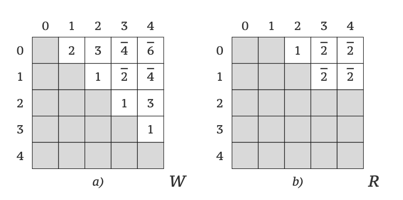
\ As we have already done previously, we are updating cells W[0,3], W[0,4], W[1,3], W[1,4] with new distances and cells R[0,3], R[0,4], R[1,3] and R[1,4] with k = 2 (see Picture 5).
\
\ There is only k = 3 left to process (because there are no edges leading from vertex 4 to any other vertex in the graph).
Again, let’s take a look at the matrix W (Picture 6).
\
\ According to the matrix W, there are three paths to vertex 3 from vertexes 0, 1 and 2 (column #3), and there is one path from vertex 3 to vertex 4 (row #3). Therefore, we have the following paths to process:
\
| Step | Path | Comment | |----|----|----| | 1 | 0 ⭢ 3 ⭢ 4 | Path found. Distance = 5 (was 6) | | 2 | 1 ⭢ 3 ⭢ 4 | Path found. Distance = 3 (was 4) | | 3 | 2 ⭢ 3 ⭢ 4 | Path found. Distance = 2 (was 3) |
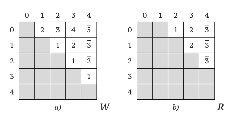
\ This was the last iteration of the algorithm. All that is left is to update cells W[0,4], W[1,4], W[2,4] with new distances and set cells R[0,4], R[1,4], R[2,4] to 3.
\ Here is what we have at the end of the algorithm (Picture 7).
\
\ As we know from the previous post, matrix W now contains all pairs of shortest paths in graph G. But what is stored inside matrix R?
HomecomingEvery time we found a new shortest path, we were updating the corresponding cell of matrix R with the current value of k. While at first, this action might look mysterious it has a very simple meaning – we were storing the vertex, from which we reached the destination vertex: i ⭢ k ⭢ j (here we are reaching j directly from k).
\ This moment is crucial. Because knowing a vertex we came from allows us to rebuild the route by moving backward (like a lobster) from the vertex j (the “to”) to vertex i (the “from”).
\ Here is a textual description of the algorithm to rebuild the route from i to j:
- Prepare empty dynamic array X.
- Start by reading a value z from cell R[i,j].
- If z is NO_EDGE, then the route from i to j is found and we should proceed to step #7.
- Prepend z to a dynamic array X.
- Read the value of cell R[i,z] into z.
- Repeat steps #3, #4, and #5 until the exit condition in #3 is reached.
- Prepend i to X.
- Append j to X.
- Now dynamic array X contains the route from i to j.
:::tip Please note, the above algorithm works only for existing paths. It also isn’t perfect from a performance point of view and for sure can be optimized. However, in the scope of this post, it is specifically described in such a way as to make it easier to understand and reproduce on a sheet of paper.
\ - Author’s note
:::
In pseudo-code, it looks even simpler:
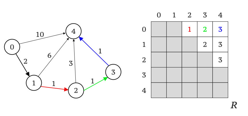
algorithm RebuildRoute(i, j, R) x = array() z = R[i,j] while (z ne NO_EDGE) do x.prepend(z) z = R[i,z] end while x.prepend(i) x.append(j) return x end algorithmLet’s try it on our graph G and rebuild a route from vertex 0 to vertex 4 (see Picture 8).
\
\ Here is a textual description of the above illustration:
We start by reading the value from R[0,4], which results in 3. According to the algorithm, this means the route goes to vertex 4 from vertex 3 (shown in BLUE).
\
Because the value of R[0,4] isn’t NO_EDGE, we proceed and read the value of R[0,3] which results in 2 (shown in GREEN).
\
Again, because the value of R[0,3] isn’t NO_EDGE, we proceed and read the value of R[0,2] which results in 1 (shown in RED).
\
At last, we read a value of R[0,1], which results in the NO_EDGE value, meaning, there are no more vertexes except 0 and 4 which contribute to the route. Therefore, the resulting route is: 0 ⭢ 1 ⭢ 2 ⭢ 3 ⭢ 4 which if you look at the graph indeed corresponds to the shortest path from vertex 0 to vertex 4.
\ A thoughtful reader might ask:
:::tip How can we be sure that all data we read from matrix R belongs to the same path?
\ - Thoughtful reader
:::
It is a very good question. We are sure because we update matrix R with a new value when we update the shortest path value in matrix W. So in the end, every row of matrix R contains data related to shortest paths. No more, no less.
\ Now, we are done with the theory, it is implementation time.
Implementation in CIn the previous post, besides implementing an original version of the Floyd-Warshall algorithm, we have also integrated various optimizations: support for sparse graphs, parallelism, and vectorization, and in the end, we also combined them all.
\ There is no reason to repeat all of this today. However, I would like to show you how to integrate route memorization into original and vectorized (with support for sparse graphs) versions of the algorithm.
Integration Into Original AlgorithmIt might be hard to believe but to integrate route memorization into the original version of the algorithms, all we need to do is to:
Extend function signature to include R matrix as a separate parameter – int[] routes.
\
Save k to routes every time the shortest path is changed (lines: 2 and 14).
\ That is it. Just one and a half lines of code:
public void BaselineWithRoutes( int[] matrix, int[] routes, int sz) { for (var k = 0; k < sz; ++k) { for (var i = 0; i < sz; ++i) { for (var j = 0; j < sz; ++j) { var distance = matrix[i * sz + k] + matrix[k * sz + j]; if (matrix[i * sz + j] > distance) { matrix[i * sz + j] = distance; routes[i * sz + j] = k; } } } } } Integration into Vectorized AlgorithmIntegration into a vectorized (with support for sparse graphs) version takes a bit more effort to complete, however, the conceptual steps are the same:
Extend function signature to include R matrix as a separate parameter – int[] routes.
\
On each iteration, initialize a new vector of k values (line: 6).
\
Save k values vector to routes every time the shortest path is changed (lines: 31-32).
\
Update a non-vectorized part of the algorithm in the same way as we updated the original algorithm (line: 41).
:::tip A small reminder – Vector.ConditionalSelect operation returns a new vector where values are equal to the smaller of two corresponding values of input vectors, i.e., if the value of vector lt_vec is equal to -1, then the operation selects a value from ij_vec, otherwise, it selects a value from k_vec.
\ - Author’s note
:::
BenchmarkingCollecting route information seems reasonable enough because… well why not? Especially when it is so easy to integrate into existing algorithms. However, let’s see how practical it is to integrate it by default.
\ Here are two sets of benchmarks: with and without (both execute original and vectorized versions of the algorithm). All benchmarks were executed by BenchmarkDotNet v0.13.1 (.NET 6.0.4 x64) on a machine equipped with an Intel Core i5-6200U CPU 2.30GHz (Skylake) processor and running Windows 10.
\ All experiments were executed on the predefined set of graphs used in the previous post: 300, 600, 1200, 2400, and 4800 vertexes.
:::info The source code and experimental graphs are available in the repository on GitHub. The experimental graphs can be found in the Data/Sparse-Graphs.zip directory. All benchmarks in this post are implemented in the APSP02.cs file.
:::
Below are the benchmark results where Baseline and BaselineWithRoutes methods correspond to the original version of the algorithm and SpartialVectorOptimisations and SpartialVectorOptimisationsWithRoutes methods correspond to a vectorized (with support for sparse graphs) version of the algorithm.
\
| Method | Size | Mean (ms) | Error (ms) | StdDev (ms) | |----|----|----|----|----| | Baseline | 300 | 40.233 | 0.0572 | 0.0477 | | BaselineWithRoutes | 300 | 40.349 | 0.1284 | 0.1201 | | SpartialVectorOptimisations | 300 | 4.472 | 0.0168 | 0.0140 | | SpartialVectorOptimisationsWithRoutes | 300 | 4.517 | 0.0218 | 0.0193 | | Baseline | 600 | 324.637 | 5.6161 | 4.6897 | | BaselineWithRoutes | 600 | 321.173 | 1.4339 | 1.2711 | | SpartialVectorOptimisations | 600 | 32.133 | 0.2151 | 0.1679 | | SpartialVectorOptimisationsWithRoutes | 600 | 34.646 | 0.1286 | 0.1073 | | Baseline | 1200 | 2,656.024 | 6.9640 | 5.8153 | | BaselineWithRoutes | 1200 | 2,657.883 | 8.8814 | 7.4164 | | SpartialVectorOptimisations | 1200 | 361.435 | 2.5877 | 2.2940 | | SpartialVectorOptimisationsWithRoutes | 1200 | 381.625 | 3.6975 | 3.2777 | | Baseline | 2400 | 21,059.519 | 38.2291 | 33.8891 | | BaselineWithRoutes | 2400 | 20,954.852 | 56.4719 | 50.0609 | | SpartialVectorOptimisations | 2400 | 3,029.488 | 12.1528 | 11.3677 | | SpartialVectorOptimisationsWithRoutes | 2400 | 3,079.006 | 8.6125 | 7.1918 | | Baseline | 4800 | 164,869.803 | 547.6675 | 427.5828 | | BaselineWithRoutes | 4800 | 184,305.980 | 210.9535 | 164.6986 | | SpartialVectorOptimisations | 4800 | 21,882.379 | 200.2820 | 177.5448 | | SpartialVectorOptimisationsWithRoutes | 4800 | 21,004.612 | 79.8752 | 70.8073 |
\ Benchmark results aren’t simple to interpret. If you take a closer look, you will find a combination when route collection actually made the algorithm run faster or without any significant effect at all.
\ This looks very confusing (and if it is – I strongly advise you to listen to this show with Denis Bakhvalov and Andrey Akinshin to better understand what tricky things can affect measurements). My best take here is that “confusing” behavior is caused by great CPU cache performance (because graphs aren’t large enough to saturate caches). Partially, this theory is based on the “bold” sample where we can see significant degradation on the largest graph. However, I didn’t verify it.
\ In general, the benchmark shows that if we aren’t talking about extremely high-performance scenarios and huge graphs, it is okay to integrate route memorization into both algorithms by default (but keep in mind, it will double memory consumption because we need to allocate two matrices W and R instead of one).
\ The only thing left is an implementation of the route rebuild algorithm.
Implementation of Route Rebuild AlgorithmImplementation of route rebuild algorithms in C# is straightforward and almost completely reflects the previously demonstrated pseudo-code (we use LinkedList
The above algorithm isn’t perfect and definitely can be improved. The simplest improvement we can make is to preallocate an array of sz size and fill it in reverse order:
public static IEnumerableWhile this “optimization” reduces the number of allocations to one, it doesn’t necessarily make the algorithm “faster” or “allocates less memory” than the previous one. The point here is if we need to have a route ordered from i to j, we always will have to “reverse” the data we retrieve from the matrix R, and there is no way to escape it.
\ But if we can present data in reverse order, then we can make use of LINQ and avoid any unnecessary allocations:
public static IEnumerableThere can be many more variants of how this code can be “changed” or “improved.” The important moment here is to remember – any “change” has downsides in terms of memory or CPU cycles.
\ Feel free to experiment! The possibilities are almost limitless!
:::info You can find implementations of all route algorithms on GitHub in the Routes.cs file.
:::
ConclusionIn this post, we had a deep dive into the theory behind the Floyd-Warshall algorithm and have extended it with the possibility of memorizing shortest paths “routes.”Then we have updated C# implementations (original and vectorized) from the previous post. In the end, we have implemented a few versions of the algorithm to rebuild the “routes”.
\ We have repeated a lot, but at the same time, I hope you have found something new and interesting in this one. This isn’t the end of the all-pairs shortest paths problem. This is just the beginning.
\ I hope you have enjoyed the reading, and see you next time!
- Home
- About Us
- Write For Us / Submit Content
- Advertising And Affiliates
- Feeds And Syndication
- Contact Us
- Login
- Privacy
All Rights Reserved. Copyright , Central Coast Communications, Inc.
