and the distribution of digital products.
How Error Coefficients Reflect Stochastic Equilibrium Expansions in Inflation Models
:::info Author:
(1) David Staines.
:::
Table of Links4 Calvo Framework and 4.1 Household’s Problem
4.3 Household Equilibrium Conditions
4.5 Nominal Equilibrium Conditions
4.6 Real Equilibrium Conditions and 4.7 Shocks
5.2 Persistence and Policy Puzzles
6 Stochastic Equilibrium and 6.1 Ergodic Theory and Random Dynamical Systems
7 General Linearized Phillips Curve
8 Existence Results and 8.1 Main Results
9.2 Algebraic Aspects (I) Singularities and Covers
9.3 Algebraic Aspects (II) Homology
9.4 Algebraic Aspects (III) Schemes
9.5 Wider Economic Interpretations
10 Econometric and Theoretical Implications and 10.1 Identification and Trade-offs
10.4 Microeconomic Interpretation
\ Appendices
A Proof of Theorem 2 and A.1 Proof of Part (i)
B Proofs from Section 4 and B.1 Individual Product Demand (4.2)
B.2 Flexible Price Equilibrium and ZINSS (4.4)
B.4 Cost Minimization (4.6) and (10.4)
C Proofs from Section 5, and C.1 Puzzles, Policy and Persistence
D Stochastic Equilibrium and D.1 Non-Stochastic Equilibrium
D.2 Profits and Long-Run Growth
E Slopes and Eigenvalues and E.1 Slope Coefficients
E.4 Rouche’s Theorem Conditions
F Abstract Algebra and F.1 Homology Groups
F.4 Marginal Costs and Inflation
G Further Keynesian Models and G.1 Taylor Pricing
G.3 Unconventional Policy Settings
H Empirical Robustness and H.1 Parameter Selection
I Additional Evidence and I.1 Other Structural Parameters
I.3 Trend Inflation Volatility
7.2 Error Coefficients
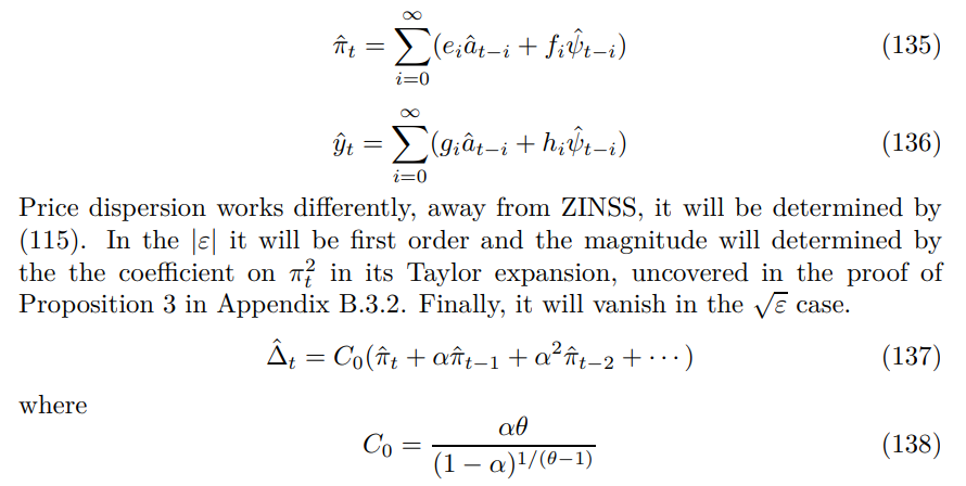
The starting point is the infinite horizon solutions, which states how present deviations depend on present and past shocks.
\
\ For the expectation variables it implies
\
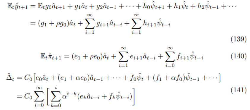
\ The first two steps remove expectations to focus on future variables. The third treats lag terms. The fourth is consolidation, the fifth deals with the Euler and the sixth puts them all together. Proceeding through the derivation in order, it is clear that
\
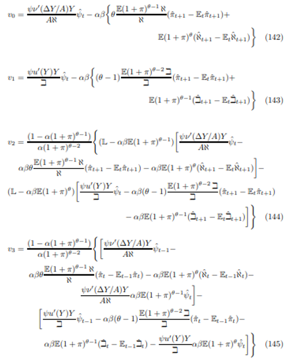
\ The coefficients have been organised so that the bracketed terms will be positive when computed in the small noise limit at strictly positive rates of trend inflation, as this is a focal alternative to ZINSS.[57] To dig down to primitives it is necessary to expand out the weighting term as follows:
\
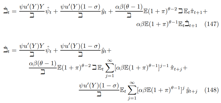
\ Expanding forward using (139), (140) and the primitive properties of the errors yields
\

\ Thus, I can substitute back into (146) to solve for the third error in terms of the canonical expansions. The unwieldy expression is suppressed. An algorithm for a solution, in terms of the stochastic equilibrium expansion coefficients, would be useful, alongside a method of numerical approximation. However, these tasks lie beyond the boundaries of this investigation.
\ The rest of the derivation is quite simple
\
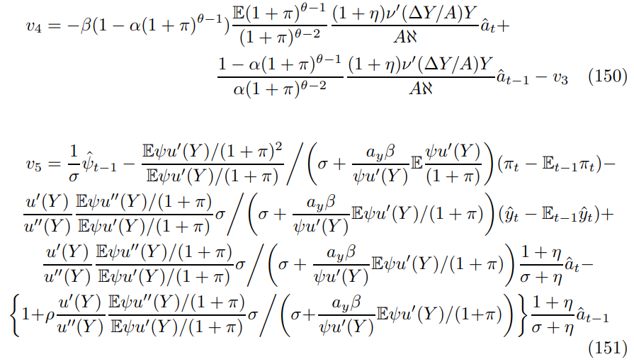
\ Combining (139), (140), (149)-(151) gives the following cumbersome expression for the Phillips curve errors
\
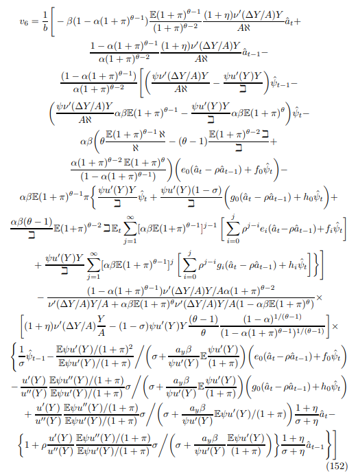
\ All subsequent error forms can be derived easily from this point.
7.2.2 Limiting Solution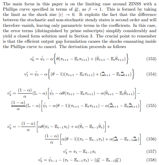
\ Now denoting the errors in (117) in the style of the slope coefficients
\

\ Hence, I am able to solve for the error coefficient using the output term in (112), the error expression (150) and the symmetry implied by (151) and (152)
\

\
:::info This paper is available on arxiv under CC 4.0 license.
:::

- Home
- About Us
- Write For Us / Submit Content
- Advertising And Affiliates
- Feeds And Syndication
- Contact Us
- Login
- Privacy
All Rights Reserved. Copyright , Central Coast Communications, Inc.