In this section, we conduct several numerical experiments to demonstrate the effectiveness of the proposed semi-implicit finite difference algorithm (Algorithm 2). Through these experiments, we examine the convergence properties of our algorithm highlighting the implementation of the fictitious play. We demonstrate that our requirement for δn in (3.3) is a sufficient yet unnecessary condition. However, in certain cases where the pure strategy equilibrium may not exist, the iteration method may not converge if the condition (3.3) is violated.

4.1 A Non-local OSMFG Example

Setup. In this example, the state of the representative agent belongs to the domain [0, 1]×R. It dynamic is a Brownian motion, i.e.

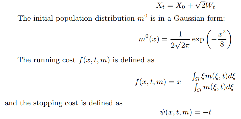
\ Intuitively, as the agent aims to minimize expected cost, the running cost encourages the agent to remain in the game when its state is below the average state of other remaining agents, while the stopping cost encourages the agent to continue playing for a longer duration.

\ It is easy to check that the cost functions above are equivalent with

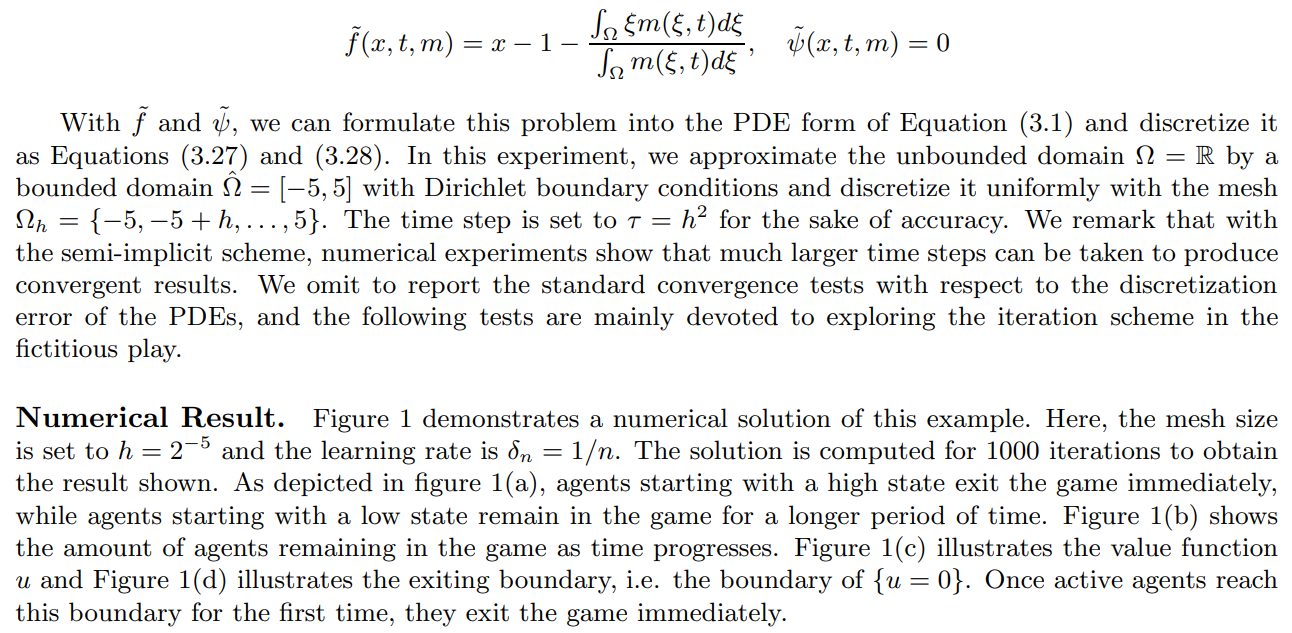
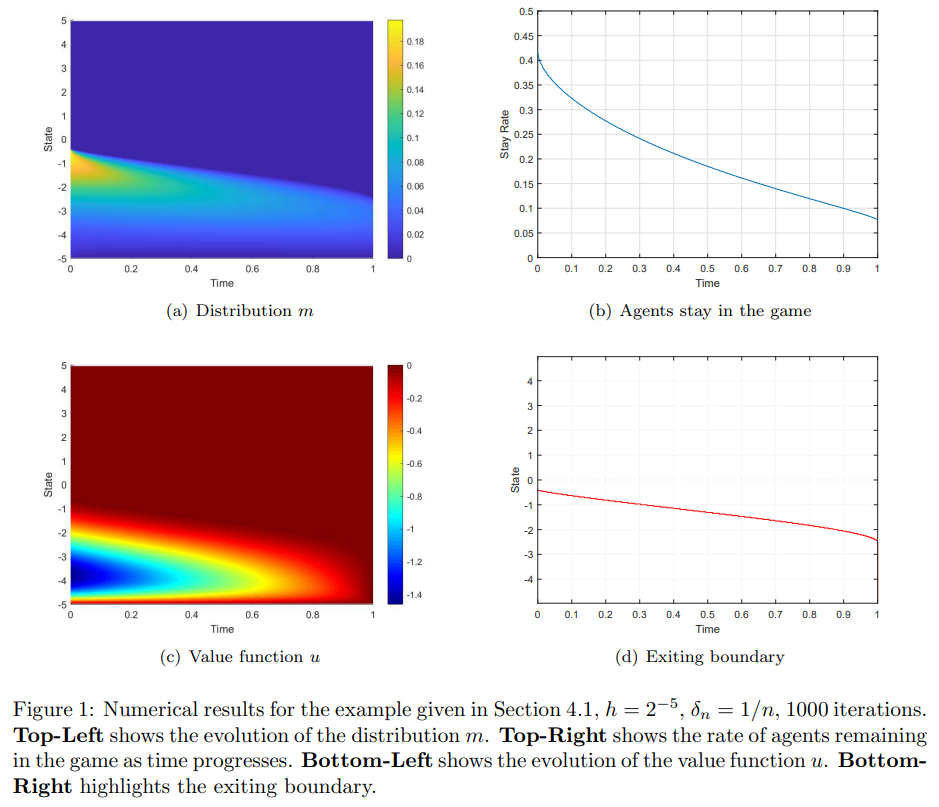
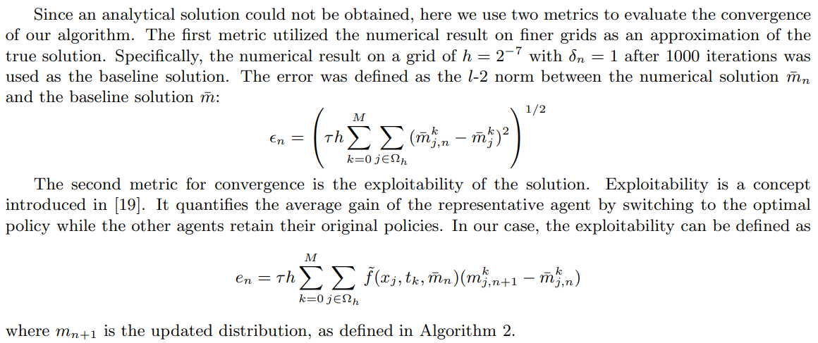
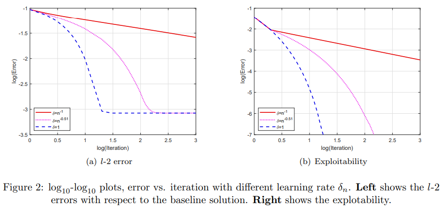
\ In Figure 2, log-log plots of error versus iteration numbers are shown for different learning rates δn. For this example, taking δn = 1 leads to the fastest convergence, although with δn = 1 no fictitious play is implemented. The reason for this is that the convergence requirement for the learning rate δn in Definition 3.1 is only a sufficient condition, rather than a necessary one. For problems with a pure strategy equilibrium, the condition in definition 3.1 can be relaxed and a more aggressive learning rate can be taken to obtain faster convergence. However, we would like to stress that we could not know a priori whether a pure strategy equilibrium exists, but the proposed algorithm, which is based on fictitious play, always produces convergence results.

:::info This paper is available on arxiv under CC 4.0 license.

:::

Feed: Hacker Noon - Medium

View: Original article