In this section, we evaluate our method on five datasets commonly adopted in multi-exit networks: MNIST [18], CIFAR-10, CIFAR-100 [16], Tiny-ImageNet [17], and ImageNet [25]. For MNIST, we

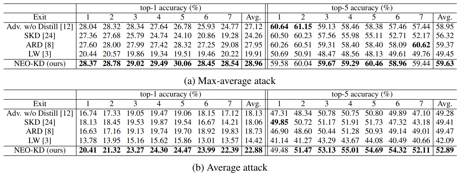
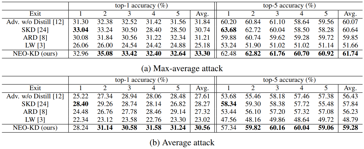
\ Adversarial test accuracy on MNIST.

\ Adversarial test accuracy on CIFAR-10.

\ use SmallCNN [12] with 3 exits. We trained the MSDNet [13] with 3 and 7 exits using CIFAR-10 and CIFAR-100, respectively. For Tiny-ImageNet and ImageNet, we trained the MSDNet with 5 exits. More implementation details are provided in Appendix.

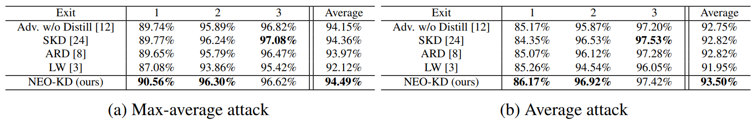
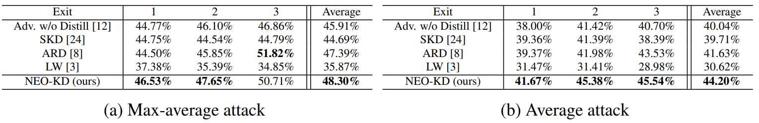
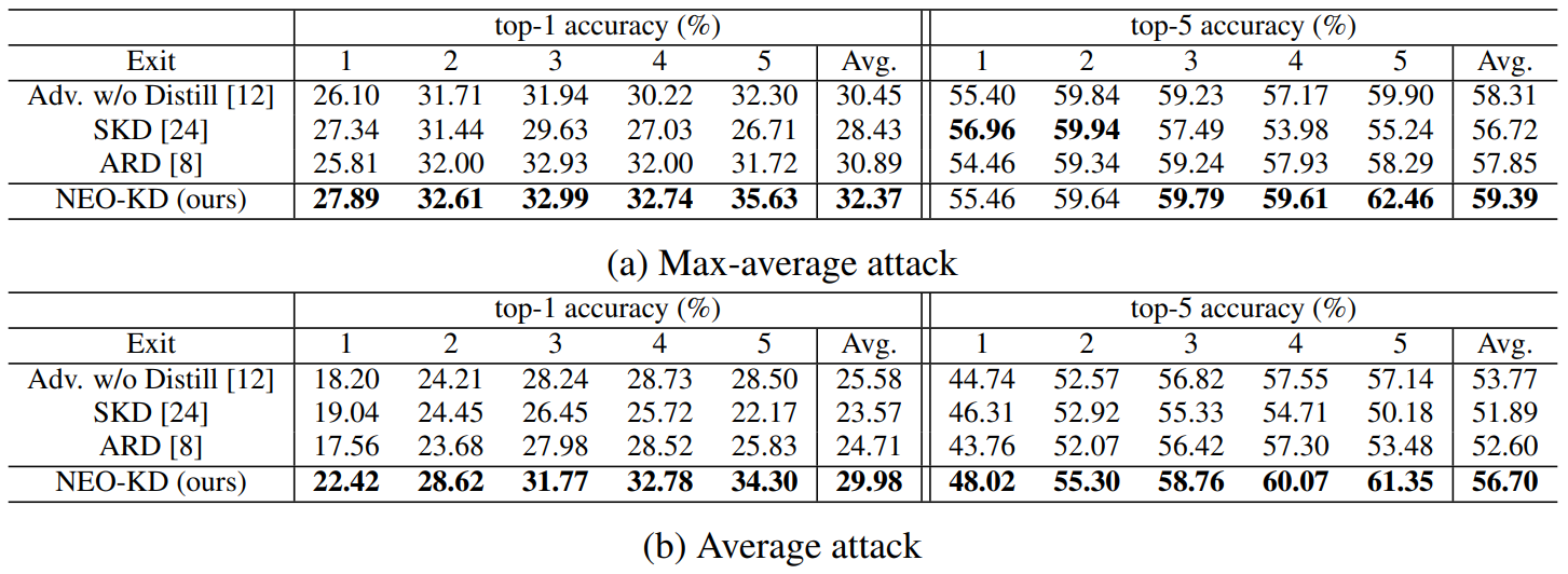
4.1 Experimental Setup

Generating adversarial examples. To generate adversarial examples during training and testing, we utilize max-average attack and average attack proposed in [12]. We perform adversarial training using adversarial examples generated by max-average attack, where the results for adversarial training via average attack are reported in Appendix. During training, we use PGD attack [21] with 7 steps as attacker algorithm to generate max-average and average attack while PGD attack with 50 steps is adopted at test time for measuring robustness against a stronger attack. We further consider other strong attacks in Section 4.3. In each attacker algorithm, the perturbation degree ϵ is 0.3 for MNIST, and 8/255 for CIFAR-10/100, and 2/255 for Tiny-ImageNet/ImageNet datasets during adversarial training and when measuring the adversarial test accuracy. Other details for generating adversarial examples and additional experiments on various attacker algorithms are described in Appendix.

\ Evaluation metric. We evaluate the adversarial test accuracy as in [12], which is the classification accuracy on the corrupted test dataset compromised by an attacker (e.g., average attack). We also measure the clean test accuracy using the original clean test data and report the results in Appendix.

\ Baselines. We compare our NEO-KD with the following baselines. First, we consider the scheme based on adversarial training without any knowledge distillation, where adversarial examples are generated by max-average attack or average attack [12]. The second baseline is the conventional self-knowledge distillation (SKD) strategy [20, 24] combined with adversarial training: during adversarial training, the prediction of the last exit for a given clean/adversarial data is distilled to the predictions of all the previous exits for the same clean/adversarial data. The third baseline is the knowledge distillation scheme for adversarial training [8], which distills the prediction of clean data to the prediction of adversarial examples in single-exit networks. As in [8], we distill the last output of clean data to the last output of adversarial data. The last baseline is a regularizer-based adversarial training strategy for multi-exit networks [3], where the regularizer restricts the weights of the fully connected layers (classifiers). In Appendix we compare our NEO-KD with the recent work TEAT [7], a general defense algorithm for single-exit networks.

\ Inference scenarios. At inference time, we consider two widely known setups for multi-exit networks: (i) anytime prediction setup and (ii) budgeted prediction setup. In the anytime prediction setup, an appropriate exit is selected depending on the current latency constraint. In this setup, for each exit, we report the average performance computed with all test samples. In the budgeted prediction setup, given a fixed computational budget, each sample is predicted at different exits depending on the predetermined confidence threshold (which is determined by validation set). Starting from the first exit, given a test sample, when the confidence at the exit (defined as the maximum softmax value) is larger than the threshold, prediction is made at this exit. Otherwise, the sample proceeds to the next exit. In this scenario, easier samples are predicted at earlier exits and harder samples are predicted at later exits, which leads to efficient inference. Given the fixed computation budget and confidence threshold, we measure the average accuracy of the test samples. We evaluate our method in these two

\ Adversarial test accuracy on CIFAR-100.

\ Adversarial test accuracy on Tiny-ImageNet.

\ Adversarial test accuracy on ImageNet.

\ settings and show that our method outperforms the baselines in both settings. More detailed settings for our inference scenarios are provided in Appendix.

:::info This paper is available on arxiv under CC 4.0 license.

:::

Feed: Hacker Noon - Medium

View: Original article

Tags: testing