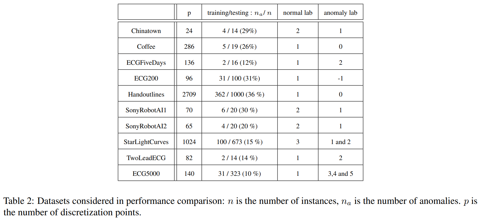
In this section, we present additional numerical experiments in support of the proposed algorithms and arguments developed in the main body of the paper. First, We describe the signature depth’s role in the algorithms and explain how this parameter affects them. We provide boxplots for two sets of generated data and argue the importance of the depth parameter in this context. Afterwards, we provide additional experiments on the robustness to noise advantage of (K)-SIF over FIF, related to Section 4.2 of the main body of the paper. The third paragraph refers to the generated data for the ’swapping events’ experiment in section 4.2 of the main body of the paper is shown. We provide a Figure for visualization and a better understanding. We further remark on how we constructed the data. The fourth subsection then demonstrates the computational time of the proposed algorithms with a direct comparison to FIF. Then, an additional experiment presenting further evidence for the discrimination power with respect to the AD task of (K)-SIF over FIF is presented. Finally, the last subsection shows a Table which describes information about the size of datasets related to the benchmark in Section 4.3.

C.1. The Role of the Signature Depth

\ In this experiment, we investigate the impact of this parameter on K-SIF with two different classes of stochastic processes. The three-dimensional Brownian motion (with µ = 0 and σ = 0.1), characterized by its two first moments, and the one-dimensional Merton-jump diffusion process, a heavy-tail process widely used to model the stock market. In such a

Algorithms

way, we compare the former class of stochastic models to the latter, which, instead, cannot be characterized by the first two moments and observe performances of (K)-SIF in this regard.

\ We computed K-SIF with three dictionaries with truncation levels varying in {2, 3, 4} for both simulated datasets. We set the number of split windows to 10, according to the previous section, and the number of trees to 1000. After that, we computed the Kendall correlation of the rank returned by these models for the three pairwise settings: level 2 vs level 3, level 2 vs level 4, and level 3 vs level 4.

\ We repeated this experiment 100 times and report the correlation boxplots in Figure 5 for the Brownian motion and in Figure 6 for the Merton-jump diffusion process. Note that the left and right plots refer to the different split window parameters selected for K-SIF, corresponding to ω = 3 for the left panels, while, for the right ones, we chose ω = 5. These boxplots show the Kendall tau correlation between the score returned by one of the algorithms used with one specific depth and the same algorithm with a different depth. K-SIF results with the three dictionaries are represented in blue, orange, and green for the Brownian, Cosine and green Gaussian wavelets, respectively. SIF boxplots are instead in purple. The y-axis refers to the Kendall correlation values and the x-axis to the settings of the depth values with respect to which the correlation has been.

\ A high correlation indicates an equivalent rank returned by the algorithm with different depth parameters. Therefore, if the correlation is high, this suggests that this parameter does not affect the results of the considered algorithm, and a lower depth should be selected for better computation efficiency. High correlations are shown for both SIF (purple boxplots) and K-SIF for the two dictionaries, i.e. Brownian and Cosine (blue and orange boxplots). Therefore, choosing the minimum truncation level is recommended to improve computational efficiency. For the same algorithms, slightly lower correlations are identified in the case of the Merton processes, yet still around 0.8 levels, hence supporting an equivalent claim. In the case of K-SIF with the Gaussian dictionary (green boxplots), a much higher variation is obtained regarding correlation results across the three tested scenarios. Furthermore, in the case of the Merton-jump diffusion processes, the results show a lower correlation, consistent with the other results. Therefore, in the case of K-SIF with such a dictionary, the depth should be carefully chosen since different parameters might lead to better detection of the moments of the underlying process.

\ ‘Brownian’ (blue), ‘Cosine’ (orange) and ‘Gaussian wavelets’ (green) on three dimensional Brownian paths.

\ ‘Brownian’ (blue), ‘Cosine’ (orange) and ‘Gaussian wavelets’ (green) with ω = 3 (left) and ω = 5 (right) on Merton-jump diffusion processes.

C.2. Robustness to Noise

This part provides additional experiments on the robustness to noise advantage of (K)-SIF over FIF, related to Section 4.2 of the main body of the paper. The configuration for data simulation goes as follows. We define a synthetic dataset of 100 smooth functions given by

\ where ε(t) ∼ N (0, 0.5). We select randomly 10% again and create slightly noisy curves by adding small noise on another sub-interval compared to the first one, i.e.,

\ where ε(t) ∼ N (0, 0.1).

\ Figure 7 provides a summary visualization of the generated dataset in the first panel. The 10 anomalous curves are plotted in red, while the 10 considered slightly noisy normal data are plotted in blue. The rest of the curves, considered normal data, is provided in gray. The idea is to understand how the dictionary choice influences K-SIF and FIF in detection of slightly noisy normal data versus abnormal noise. Results for K-SIF and FIF are provided in the second, third and fourth panels of Figure 7, respectively.

\ We compute K-SIF with a Brownian dictionary, k = 2 and ω = 10 and FIF for α = 0 and α = 1 also with a Brownian dictionary. The colors of the panels represent the anomaly score assigned to each curve for that specific algorithm. In the second (K-SIF) and last (FIF with α = 0) panels, the anomaly score increases from yellow to dark blue, i.e. a dark curve is abnormal and yellow is normal, while, in the third plot (FIF with α = 1) it is the opposite, i.e. a dark curve is normal and yellow is abnormal.

\ It is possible to observe how K-SIF successfully can identify noisy and abnormal data as such. Indeed, while the abnormal data are colored in dark blue, the noisy ones display a yellow color score. Instead, in FIF with α = 1 (third panel) both the abnormal and the slightly noisy curves are identified as normal data (given the reversed scale and having dark blue colors). When it comes to FIF with α = 0 (last and fourth panel), both abnormal and noisy data are scored as abnormal curves. Hence, FIF with both settings of the α parameter, cannot provide a different score to noise and slightly noisy data. K-SIF, instead, successfully perform such a task.

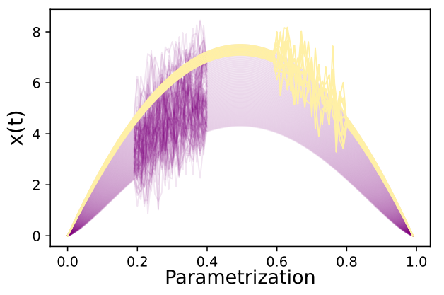
C.3. Swapping Events Dataset

This part provides a visualization of the dataset used in the ‘swapping events’ experiment in section 4.2 of the core paper. Figure 8 shows the simulated data. Remark that we define a synthetic dataset of 100 smooth functions given by

\ with t ∈ [0, 1] and q equispaced in [1, 1.4]. Then, we simulate the occurrences of events by adding Gaussian noise on different portions of the functions. We randomly select 90% of them and add Gaussian values on a sub-interval, i.e.,

\ where ε(t) ∼ N (0, 0.8). We consider the 10% remaining as abnormal by adding the same ‘events’ on another sub-interval compared to the first one, i.e.,

\ where ε(t) ∼ N (0, 0.8). We then have constructed two identical events occurring at different parts of the functions, leading to isolating anomalies.

\ Swapping Events. Dataset used in the experiment of Section 4.2. Purple curves represent normal data whileyellow curves represent abnormal data. Configuration of the simulation are provided at the beginning of the section.

C.4. Computational Time of K-SIF, SIF and FIF

\ Computational time for K-SIF and FIF with respect to the number of curves (left), the number of discretization points (middle) and the number of dimension (right).

C.5. K-SIF and SIF: a Better Discrimination of Anomalies compared to FIF

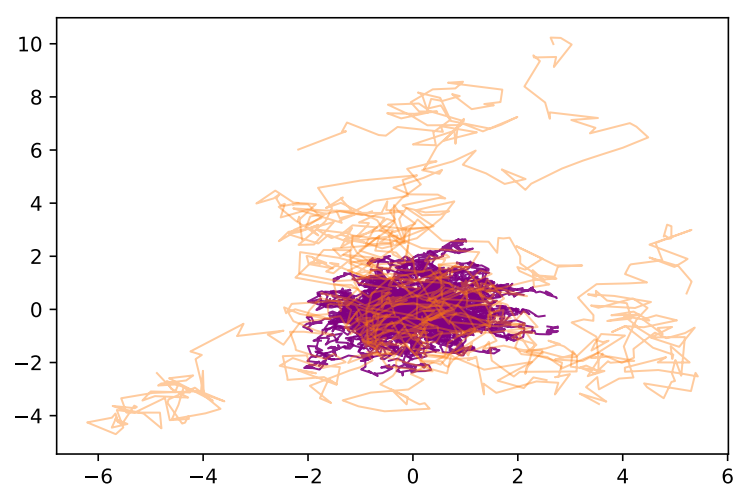
In this part, we construct an additional toy experiment to show the discrimination power of (K-)SIF over FIF. We simulate 100 planar Brownian motion paths with 90% of normal data with drift µ = [0, 0] and standard deviation σ = [0.1, 0.1], and 10% of abnormal data with drift µ = [0, 0] and standard deviation σ = [0.4, 0.4].

\ Figure 10 presents one simulation of this dataset. Note that, the purple paths represent normal data, while, in orange, the abnormal are instead represented. On this dataset, we compute FIF (with α = 1 and Brownian dictionary), K-SIF (with

\ Dataset used for the experiment. Purple paths are normal data while orange paths are the abnormal ones.

\ k = 2, ω = 10 and Brownian dictionary) and SIF (with k = 2 and ω = 10). To display the scores returned by the algorithsm, we provide Figure 11. Note that, the plots shows the scores for these 100 paths, after having sorted them. Hence, the x-axis provides the index of the ordered scores, while, the y-axis represents the score values. As for the simulation, we plot in purple the scores of the normal data and in orange the scores of the abnormal data. The three panels refer to FIF, K-SIF and SIF, respectively.

\ It is possible to observe that the scores of K-SIF and SIF well separate the abnormal and the normal data, with a jump in the scores which is quite pronounced, i.e. the scores of the normal data are relatively distant from the scores of the abnormal data. If one focuses on FIF instead, then the discrimination of such anomalies appears to be more challenging; the first panel shows, in fact, a continuous in terms of the score returned by the AD algorithm, which does not separate normal and abnormal data.

\ In summary, the proposed algorithms leveraging the signature kernel (K-SIF) and the signature coordinate (SIF) exhibit more reliable results in this experimental setting, suggesting their efficacy in discerning anomalies within the simulated dataset. Detecting the order in which events happen is a much more informative feature than incorporating a functional aspect in the anomaly detection algorithm. This aspect must be further investigated and explored, particularly in the application areas where sequential data, such as time series, are taken into account.

\ Scores returned by FIF (left), K-SIF (middle) and SIF (right) on planar Brownian motion with abnormal data (orange).

C.6. Anomaly Detection Benchmark Data

C.7. Background on Data Depth function

Statistical tools known as data depths serve as intrinsic similarity scores in this context. Data depths offer a straightforward geometric interpretation, ordering points from center outward with respect to a probability distribution (Tukey, 1975; Zuo and Serfling, 2000). Geometrically, data depths gauge the depth of a sample within a given distribution. Despite garnering attention from the statistical community, data depths have been largely overlooked by the machine learning community. Numerous definitions have been proposed, as alternatives to the earliest proposal, the halfspace depth introduced in (Tukey, 1975). Among many others these include: the simplicial depth (Liu, 1988), the projection depth (Liu and Singh, 1993), the zonoid depth (Koshevoy and Mosler, 1997), the regression depth (Rousseeuw and Hubert, 1999), the spatial depth (Vardi and Zhang, 2000) or the AI-IRW depth (Clemen ´ c¸on et al., 2023) differing in their properties and applications. Data depth finds many applications such as defining robust metrics between probability distribution (Staerman et al., 2021b) competing with robust optimal transport based metrics (Staerman et al., 2021a), finding adversarial attacks in computer vision (Picot et al., 2022; Dadalto et al., 2023) or detecting hallucination in NLP transformers (Colombo et al., 2023; Darrin et al., 2023; Colombo et al., 2022) and LLM (Himmi et al., 2024).

:::info This paper is available on arxiv under CC BY 4.0 DEED license.

:::

Feed: Hacker Noon - Medium

View: Original article

Tags: application applications distribution small stock underlying